Fieldline plot
Before starting this section make sure to have a camera set up. Also if there’s a bounding box in the scene, it’s generally easier to navigate and understand the directions in space. So before moving forward, check previous tutorial on basics of BRender. Also since we’re going to do a plot fieldlines, it’s a good idea to have either volumetric or particle data plotted before moving forward (see previous sections for that).
Note
for tigressdata users. Blender’s bundled python does not support hdf5 documents, and I wasn’t able to install it (no access). So you’ll have to do all the reading and primary analysis of all the data from some python outside Blender.
Generating fieldlines
To generate streamlines we here use a custom method that was generalized for 3D case from matplotlib’s streamplot function. I’m not going to describe it here in details, the only thing to have in mind is that you’ll have to specify several parameters before generating fieldlines.
keys(default:('bx', 'by', 'bz')) - the field keys that will be taken fromhdf5as a vector field.density(default:1) - very similar to that instreamplot, a parameter that determines how dense are the fieldlines.n_traj(default:100) - total number of fieldline trajectories.seg_step(default:0.2) - integration step (in simulation units); make sure to keep it less than 1.min_seglen(default:100.) - minimum fieldline length (in simulation units).region(point)(default:True) - function that takes as argument the tuple of(x,y,z)coordinates (in simulation units) and returns a logical expression that determines which constraints the region of fieldlines.
Let’s define all those variables in a following manner (for tigressdata do this outside Blender):
fname = '/path-to/flds.tot.001'

density = 2.
n_traj = 50
seg_step = 0.8
min_seglen = 100

def region(point):
    x, y, z = point
    # this means only the region with 400 < x < 600 will be considered
    return (x > 400 and x < 600)
To generate trajectories we’ll first need to import the module and then use generateFieldlines() function:
import lib.export_trajectories as fldlns

trajectories = fldlns.generateFieldlines(fname, density = density, keys = ('bx', 'by', 'bz'),
                                                n_traj = n_traj, region = region, min_seglen = min_seglen,
                                                seg_step = seg_step)
Now each of trajectories[i] array contains all the fieldlines in the following form:
x1  y1  z1
x2  y2  z2
...
xN  yN  zN
Note
If you’re doing this in tigressdata you’ll have to save those trajectories to later import them from inside Blender. Do:
out_file = '/path-to/fieldlines.dat'
fldlns.exportFieldlines(trajectories, out_file)
Plotting fieldlines
If you’re working in Mac you will simply have your fieldlines in the trajectories variable. You’ll also need to know the shape and scale of your simulation box:
import numpy as np # if not yet imported
import lib.to_bvox as bvox

fname = '/path-to/flds.tot.001'
shape0 = np.array(bvox.getShape(fname, 'dens'))
scale = 2. / shape0.min()
shape = shape0 * scale
If you’re working within tigressdata, you’ll have to specify shape and size manually (e.g. by running the code above from outside Blender and then printing and copy-pasting values). The trajectories can be imported from the .dat filed saved above (make sure to have import brender as br):
out_path = '/path-to/fieldlines.dat'
trajectories = br.importFieldlines(out_path)
Now with either system, simply run (make sure to have import brender as br):
fieldlines = br.FieldLines(trajectories, name = 'b-field', size = shape, scale = scale)
This will create a FieldLines object with the given fieldlines. You can later configure color and intensity:
fieldlines.color = '#123123'
fieldlines.intensity = 0.5
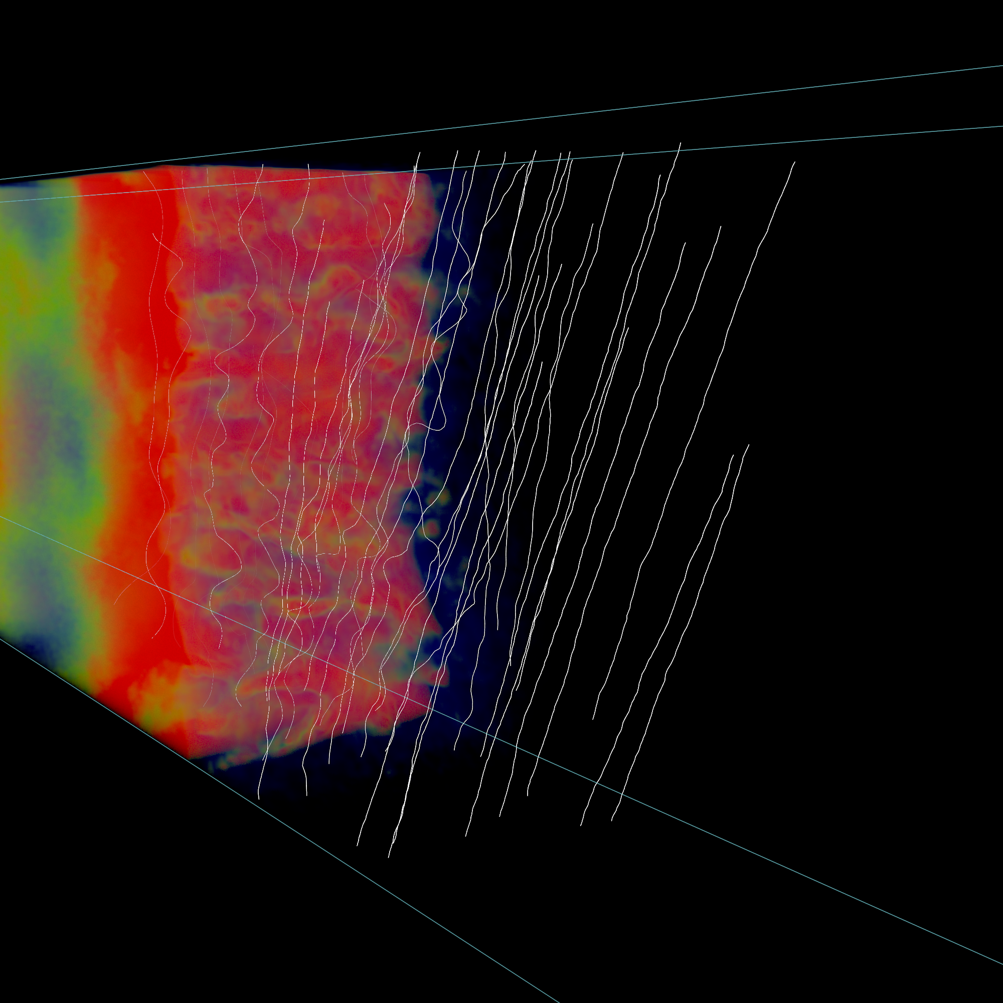
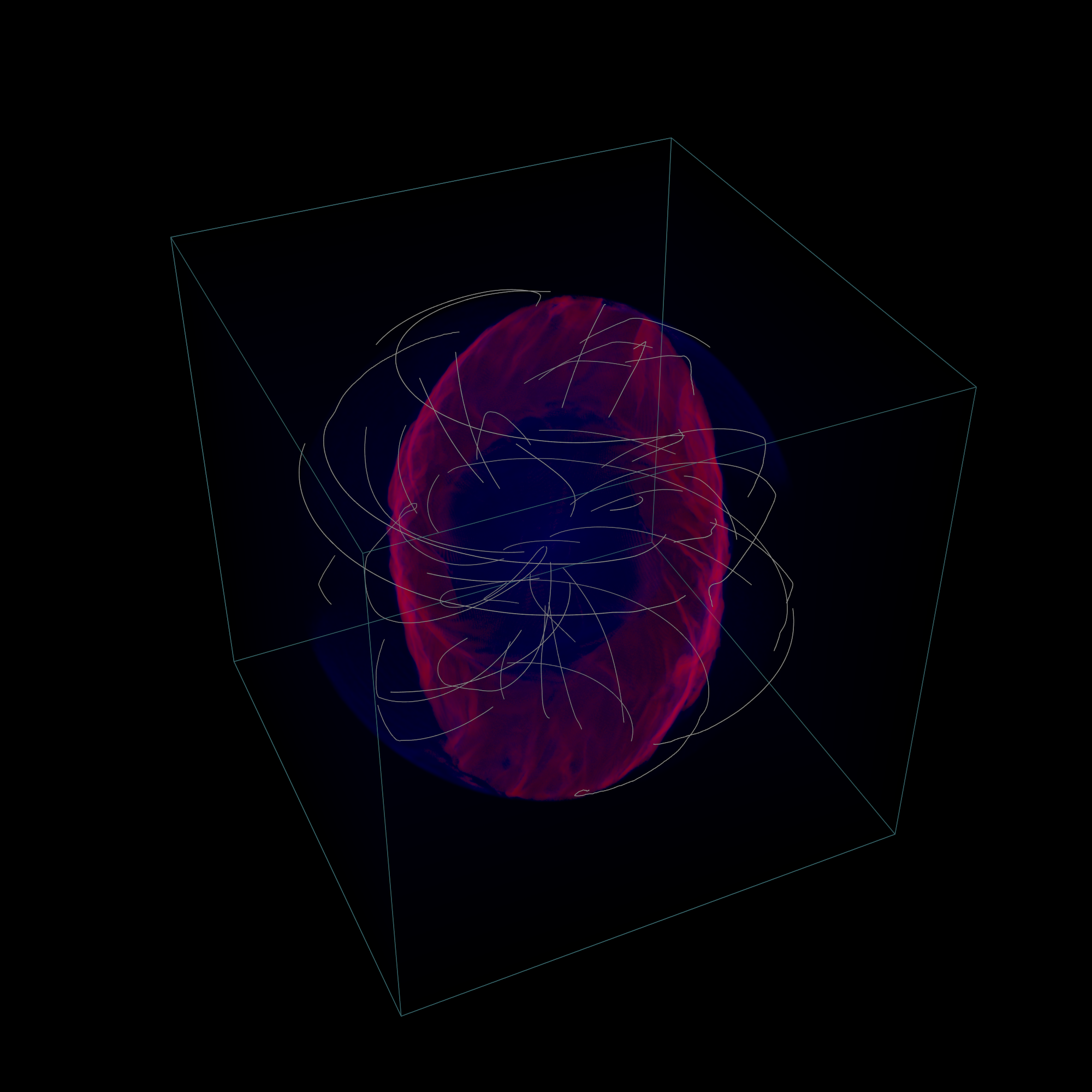
Below are two rendering results.
Full python script
for Mac
"""Example code to run within Blender to produce the plot show above (Mac version)

    Note: Make sure to change all the paths below

"""

import brender as br

# # # # # # # # # # # # # # # # # # # # # # # #
#
#   1. Preparing
#
# # # # # # # # # # # # # # # # # # # # # # # #
# setting up the camera
cam = br.initializeCamera()
cam.location = (4.5, -1.2, 0.7)
cam.pointing = (0, 0, 0)

# setting up the renderer
render_directory = '/any-folder/images/'
render_name = 'mysim_'
render = br.Render(render_directory, render_name)

br.Render.set_resolution(1000, 1000)

import lib.to_bvox as bvox
import numpy as np

# finding the shape and scale of our simulation
fname = '/path-to/flds.tot.001' # <-- this is for TRISTAN
shape0 = np.array(bvox.getShape(fname, 'dens'))
scale = 2. / (shape0.min())
shape = shape0 * scale

# # # # # # # # # # # # # # # # # # # # # # # #
#
#   2. Generating .bvox file
#       if the .bvox already exists, just skip this step
#
# # # # # # # # # # # # # # # # # # # # # # # #
density = 0.5
n_traj = 50
seg_step = 0.2
min_seglen = 60

def region(point):
    x, y, z = point
    # this means only the region with 400 < x < 600 will be considered
    return (x > 400) and (x < 600)

import lib.export_trajectories as fldlns

trajectories = fldlns.generateFieldlines(fname, density = density, keys = ('bx', 'by', 'bz'),
                                                n_traj = n_traj, region = region, min_seglen = min_seglen,
                                                seg_step = seg_step)

# # # # # # # # # # # # # # # # # # # # # # # #
#
#   3. Plotting
#
# # # # # # # # # # # # # # # # # # # # # # # #
# generating the FieldLines class object
fieldlines = br.FieldLines(trajectories, name = 'b-field', size = shape, scale = scale)

# adjusting intensity, etc
fieldlines.intensity = 0.2
fieldlines.color = (0,1,1)

# ...and finally rendering (or use Fn+F12)
render.render()
# image saved to the directory defined above
for tigressdata
outside Blender:
"""Example code to run outside Blender (tigressdata version)

    Note: Make sure to change all the paths below
    Note2: This is to be run outside Blender

"""
import sys
import numpy as np
sys.path.append('/path-to-brender-repo') # you can use mine: '/home/hakobyan/Downloads/brender_astro'
import lib.to_bvox as bvox
import lib.export_trajectories as fldlns

# # # # # # # # # # # # # # # # # # # # # # # #
#
#   1. Preparing
#
# # # # # # # # # # # # # # # # # # # # # # # #
fname = '/path-to/flds.tot.001'
shape0 = np.array(bvox.getShape(fname, 'dens'))
scale = 2. / (shape0.min())
shape = shape0 * scale

# you need to copy this parameters later
print (shape)
print (scale)

# # # # # # # # # # # # # # # # # # # # # # # #
#
#   2. Generating .dat file with trajectories
#
# # # # # # # # # # # # # # # # # # # # # # # #
fname = '/path-to/flds.tot.001'

density = 0.5
n_traj = 50
seg_step = 0.2
min_seglen = 60

def region(point):
    x, y, z = point
    # this means only the region with 400 < x < 600 will be considered
    return (x > 400) and (x < 600)

import lib.export_trajectories as fldlns

trajectories = fldlns.generateFieldlines(fname, density = density, keys = ('bx', 'by', 'bz'),
                                                n_traj = n_traj, region = region, min_seglen = min_seglen,
                                                seg_step = seg_step)

out_file = '/path-to/fieldlines.dat'
fldlns.exportFieldlines(trajectories, out_file)
inside Blender:
"""Example code to run inside Blender (tigressdata version)

    Note: Make sure to change all the paths below
    Note2: This is to be run inside Blender, we do not refer to h5py here

"""

# # # # # # # # # # # # # # # # # # # # # # # #
#
#   1. Preparing
#
# # # # # # # # # # # # # # # # # # # # # # # #
# setting up the camera
cam = br.initializeCamera()
cam.location = (4.5, -1.2, 0.7)
cam.pointing = (0, 0, 0)

# setting up the renderer
render_directory = '/any-folder/images/'
render_name = 'mysim_'
render = br.Render(render_directory, render_name)

br.Render.set_resolution(1000, 1000)

# # # # # # # # # # # # # # # # # # # # # # # #
#
#   2. Plotting
#
# # # # # # # # # # # # # # # # # # # # # # # #
out_path = '/path-to/fieldlines.dat'
field_data = br.importFieldlines(out_path) # importing trajectories

# set `shape` and `scale` manually below
fieldlines = br.FieldLines(field_data, name = 'b-field', size = shape, scale = scale)

# adjusting intensity, etc
fieldlines.intensity = 0.2
fieldlines.color = (0,1,1)