Particle plot
Before starting this section make sure to have a camera set up. Also if there’s a bounding box in the scene, it’s generally easier to navigate and understand the directions in space. So before moving forward, check previous tutorial on basics of BRender.
Note
for tigressdata users. Blender’s bundled python does not support hdf5 documents, and I wasn’t able to install it (no access). So you’ll have to do all the reading and primary analysis of all the data from some python outside Blender.
Generating particle coordinates
Again, similar to the previous section, BRender is not constrained to any specific code output, and can be fed by any sort of particle data generated in advance. So if you know how to generate a set of coordinates kept in an array from a specific code output, feel free to skip to the next section where we’ll be making a particle plot.
Here we’ll discuss how to generate particle array particularly for TRISTAN code output (hdf5 format), which will be later used to make a plot. Note again, that if you’re working from within the tigressdata, you’ll have to do this from a python outside Blender, Mac users can do this from inside Blender console. We first need to specify several paths and names:
# For tigressdata do this whole procedure from outside Blender python console
import lib.particle_output as prtl

out_path = '/output-dir-for-particles/' # <-- make sure to have slash in the end
fpart = '/path-to/prtl.tot.001' # <-- this one is specifically a TRISTAN output file

n_particles = 20000 # number of particles per each sort
For the particle output, you need to somehow tell the function what’s the physical shape of your simulation (in units of code). For that, it either takes the values from the param.*** file from the same location as the prtl.tot.*** file, or it takes it from flds.tot.*** (then you’ll have to provide it with istep value), or you can also specify it manually with the shape attribute (the function will take care of it):
# in this case I have the `flds.tot.001` in the same location, so I only provide the `istep`
fpath = prtl.makeParticles(out_path, fpart, n_particles, istep = 4)
This will create a particles.dat file in the location given by out_path with an array of particles: (x, y, z, ind), where ind being the index of a particle (0 for electrons and 1 for ions) and x, y, z being the coordinates of a random sample of n_particles particles scaled so the smallest edge is 2 (with the center in (0,0,0)). The typical output looks like this:
# content of `particles.dat`
...
 0.0632148981094     -0.047459602356      0.227420449257      0.0
-0.0733104348183     -0.135616958141      0.0196393728256     0.0
 0.437074899673       0.260051727295      0.24244260788       0.0
 0.0026843547821     -0.0520194172859    -0.214550793171      0.0
-0.21538990736       -0.138226926327      0.0670219659805     0.0
...
-0.160959780216      -0.0728992819786     0.0648549795151     1.0
 0.0687325000763      0.0521985292435    -0.0412805080414     1.0
-0.0846030116081      0.332876563072     -0.349565148354      1.0
-0.00664752721786    -0.320498406887     -0.0523825287819     1.0
-0.414578616619       0.0203070640564     0.0408389568329     1.0
...
In the next section we will import this data and feed it to a class that creates the particle plot.
Making particle plot
Note
For tigressdata the rest can be done within the Blender console.
The only data you need to have is an array of (x, y, z) coordinates scaled within a given shape (it’s convenient to have a min edge size of 2). If you have those arrays (as many as you like depending on how many particle species you have), skip to the step 2.
If you working within tigressdata, specify a path to particles.dat file:
fpath = '/path-to/particles.dat'
We will then import the particle data, split the particles into different arrays according to their indices (if necessary):
import numpy as np

xs, ys, zs, inds = np.loadtxt(fpath, unpack=True, usecols=(0,1,2,3))

# electrons with `ind` = 0
xs_e = xs[inds == 0]
ys_e = ys[inds == 0]
zs_e = zs[inds == 0]
coords_e = list(zip(xs_e, ys_e, zs_e))
# ions with `ind` = 1
xs_i = xs[inds == 1]
ys_i = ys[inds == 1]
zs_i = zs[inds == 1]
coords_i = list(zip(xs_i, ys_i, zs_i))
You then can make two objects that will have your particle plots for both electrons and ions:
# blue electrons
part_lec = br.ParticlePlot(coords_e, name = 'lecs', halo_size = 0.005, color = (0, 0, 1))
# red electrons
part_ion = br.ParticlePlot(coords_e, name = 'ions', halo_size = 0.005, color = (1, 0, 0))
The halo_size parameter sets the characteristic “particle size”. You can later adjust color, location and scale (with respect to your original coords scaling) by doing (e.g.):
part_lec.color = '#123123'
part_lec.location = (-0.5, 0.2, 0.3)
part_lec.halo_size = 0.001
part_lec.scale = 2. # this will inflate the data cube twice
One can also redraw the whole thing with updated coordinates (stored in coords_new) by doing:
part_lec.coords = coords_new
Note
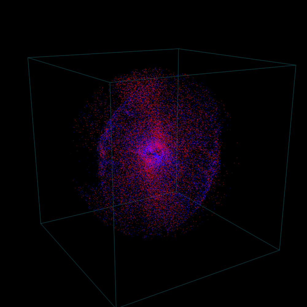
You can always play with all the parameters from the Blender GUI (see below).
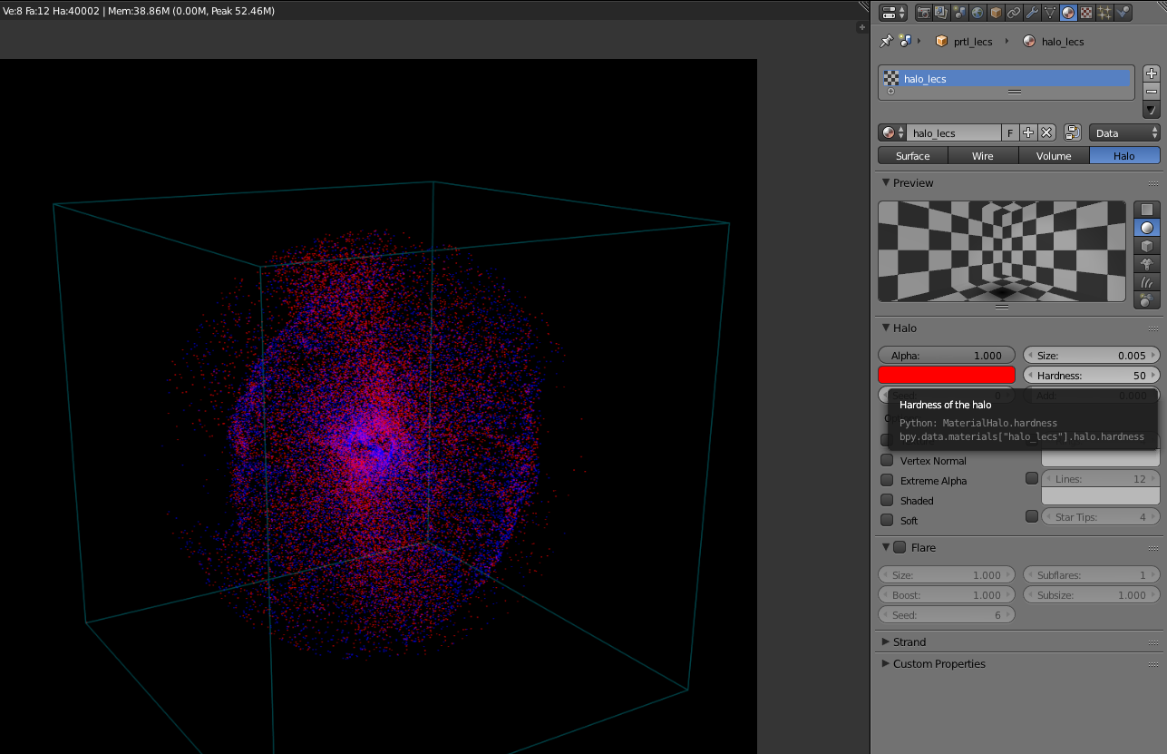
Below is a rendering result of such a plot.
Full python script
for Mac
"""Example code to run within Blender to produce the plot show above (Mac version)

    Note: Make sure to change all the paths below

"""

import brender as br

# # # # # # # # # # # # # # # # # # # # # # # #
#
#   1. Preparing
#
# # # # # # # # # # # # # # # # # # # # # # # #
# setting up the camera
cam = br.initializeCamera()
cam.location = (4.5, -1.2, 0.7)
cam.pointing = (0, 0, 0)

# setting up the renderer
render_directory = '/any-folder/images/'
render_name = 'mysim_'
render = br.Render(render_directory, render_name)

br.Render.set_resolution(1000, 1000)

import lib.particle_output as prtl

out_path = '/output-dir-for-particles/' # <-- make sure to have slash in the end
fpart = '/path-to/prtl.tot.001' # <-- this one is specifically a TRISTAN output file

n_particles = 20000 # number of particles per each sort

# # # # # # # # # # # # # # # # # # # # # # # #
#
#   2. Generating `particles.dat` file
#       You can skip this, if you already have the particles' (x,y,z) loaded into an array
#
# # # # # # # # # # # # # # # # # # # # # # # #
# in this case I have the `flds.tot.001` in the same location, so I only provide the `istep`
fpath = prtl.makeParticles(out_path, fpart, n_particles, istep = 4)

# reading everything to 2 arrays
import numpy as np

xs, ys, zs, inds = np.loadtxt(fpath, unpack=True, usecols=(0,1,2,3))

# electrons with `ind` = 0
xs_e = xs[inds == 0]
ys_e = ys[inds == 0]
zs_e = zs[inds == 0]
coords_e = list(zip(xs_e, ys_e, zs_e))
# ions with `ind` = 1
xs_i = xs[inds == 1]
ys_i = ys[inds == 1]
zs_i = zs[inds == 1]
coords_i = list(zip(xs_i, ys_i, zs_i))

# # # # # # # # # # # # # # # # # # # # # # # #
#
#   3. Plotting
#
# # # # # # # # # # # # # # # # # # # # # # # #
# blue electrons
part_lec = br.ParticlePlot(coords_e, name = 'lecs', halo_size = 0.005, color = (0, 0, 1))
# red electrons
part_ion = br.ParticlePlot(coords_e, name = 'ions', halo_size = 0.005, color = (1, 0, 0))
for tigressdata
outside Blender:
"""Example code to run outside Blender (tigressdata version)

    Note: Make sure to change all the paths below
    Note2: This is to be run outside Blender

"""

import sys
sys.path.append('/path-to-brender-repo') # you can use mine: '/home/hakobyan/Downloads/brender_astro'
import lib.particle_output as prtl

# # # # # # # # # # # # # # # # # # # # # # # #
#
#   Generating `particles.dat` file
#       You can skip this, if you already have the particles' (x,y,z) loaded into an array
#
# # # # # # # # # # # # # # # # # # # # # # # #

out_path = '/output-dir-for-particles/' # <-- make sure to have slash in the end
fpart = '/path-to/prtl.tot.001' # <-- this one is specifically a TRISTAN output file

n_particles = 20000 # number of particles per each sort

# in this case I have the `flds.tot.001` in the same location, so I only provide the `istep`
fpath = prtl.makeParticles(out_path, fpart, n_particles, istep = 4)
inside Blender:
"""Example code to run inside Blender (tigressdata version)

    Note: Make sure to change all the paths below
    Note2: This is to be run inside Blender, we do not refer to h5py here

"""

# # # # # # # # # # # # # # # # # # # # # # # #
#
#   1. Preparing
#
# # # # # # # # # # # # # # # # # # # # # # # #
# setting up the camera
cam = br.initializeCamera()
cam.location = (4.5, -1.2, 0.7)
cam.pointing = (0, 0, 0)

# setting up the renderer
render_directory = '/any-folder/images/'
render_name = 'mysim_'
render = br.Render(render_directory, render_name)

br.Render.set_resolution(1000, 1000)

# # # # # # # # # # # # # # # # # # # # # # # #
#
#   2. Reading `particles.dat` file
#       You can skip this, if you already have the particles' (x,y,z) loaded into an array
#
# # # # # # # # # # # # # # # # # # # # # # # #

fpath = '/path-to/particles.dat'

# reading everything to 2 arrays
import numpy as np

xs, ys, zs, inds = np.loadtxt(fpath, unpack=True, usecols=(0,1,2,3))

# electrons with `ind` = 0
xs_e = xs[inds == 0]
ys_e = ys[inds == 0]
zs_e = zs[inds == 0]
coords_e = list(zip(xs_e, ys_e, zs_e))
# ions with `ind` = 1
xs_i = xs[inds == 1]
ys_i = ys[inds == 1]
zs_i = zs[inds == 1]
coords_i = list(zip(xs_i, ys_i, zs_i))

# # # # # # # # # # # # # # # # # # # # # # # #
#
#   3. Plotting
#
# # # # # # # # # # # # # # # # # # # # # # # #

# blue electrons
part_lec = br.ParticlePlot(coords_e, name = 'lecs', halo_size = 0.005, color = (0, 0, 1))
# red electrons
part_ion = br.ParticlePlot(coords_e, name = 'ions', halo_size = 0.005, color = (1, 0, 0))