Basics of BRender¶

Now that we have everything set up and have Blender windows open with console and pre-loaded python script, let’s try to do some basics. In principle, anything done below can be done without coding at all by using the Blender GUI. However, sometimes it is much faster and easier to do things using simple scripts.

First in the console do:

import brender as br

This will import BRender module with all the functions.

Camera¶

Let’s first create a camera and an empty object which will serve as a flag where the camera will be pointing:

cam = br.initializeCamera()

Now cam contains the camera object and the related empty object. By default camera will have a particular location, which can be changed by doing:

cam.location = (3.2, -2.5, 1.4)

We can also adjust where the direction at which camera is pointing:

cam.pointing = (0.4, 1., 1.)

This might be handy when doing an animation and need a complex camera motion. Other options to play around with:

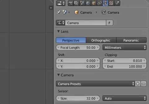
cam.type = 'PERSP' # 'ORTHO', 'PANO' # <- this is camera type
cam.lens = 50 # <- focal length for type 'PERSP' camera type only
cam.ortho_scale = 3.5 # <- orthographic scale for type 'ORTHO' camera type only

Note

If you want to explore the attributes further, feel free to navigate cursor on different parameters in the Properties bar. When hovering over, Blender will show the python script for the attribute, such as bpy.data.cameras['Camera'].type, where bpy.data.cameras['Camera'] is our cam object.

Viewport navigation¶

This part is strictly GUI based. Usually the navigation in the 3d viewport is being done by numpad keys, however most of the people don’t have numpads.

Mac users¶

On mac the easiest way of navigation is via trackpad. Standard gestures are:

two-finger pinch (for zoom)
swipe (for rotate)
Shift + swipe (for move)

Mouse gestures:

middle mouse scroll (for zoom)
middle mouse + move (for rotate)
Shift + middle mouse + move (for move)

These gestures can be configured from inside Blender: File -> User Preferences (Cmd+,), from the Input tab find 3D View and then 3D View (Global) dropdown menu. Then click Save User Settings below.

Tigressdata users¶

On tigressdata (via vnc) Mac trackpad gestures do not work. So you will either need to have a mouse with the same gestures (see above), or you can configure gestures

These gestures can be configured from inside Blender: File -> User Preferences (Ctrl+Alt+U), from the Input tab find 3D View and then 3D View (Global) dropdown menu. Adjust:

Set 3D Cursor set to something else
Rotate View set Left Mouse
Move View set Shift Left Mouse

Again, click Save User Settings. Now you can rotate and move with a simple trackpad click.

Note

You can also just copy my userpref.blend file from here (/home/hakobyan/.config/blender/2.76/config/) and paste it to your (/home/<username>/.config/blender/2.76/config/) directory. If the directory doesn’t exist, create it.

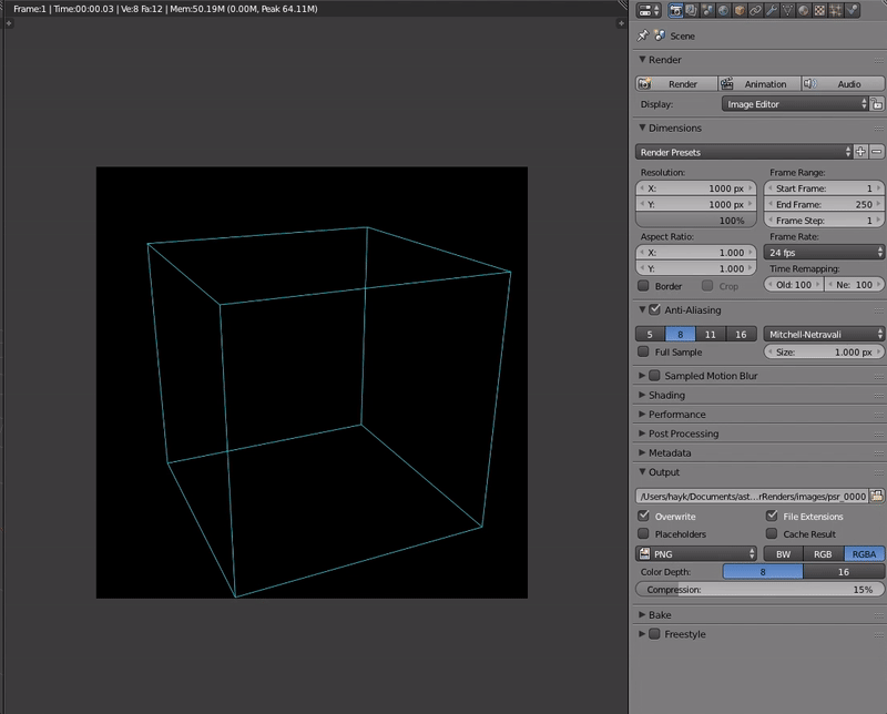
Rendering¶

Let us first assign a render directory and a desired tag-name for the rendered images:

render_directory = '/directory-of-choice/'
name = 'plot_'
render = br.Render(render_directory, render_name)

Now if we want to render an image from the active camera we simply run:

render.render()

This is handy if we’re doing multiple shots, but if we just want to look at a single snapshot, it’s probably easier to press F12 (fn+F12 for Mac) for quick render. The result will be shown in one of the Blender windows.

We can also change the resolution of our render by doing:

br.Render.set_resolution(1000, 1000) # <- these are the values I usually use

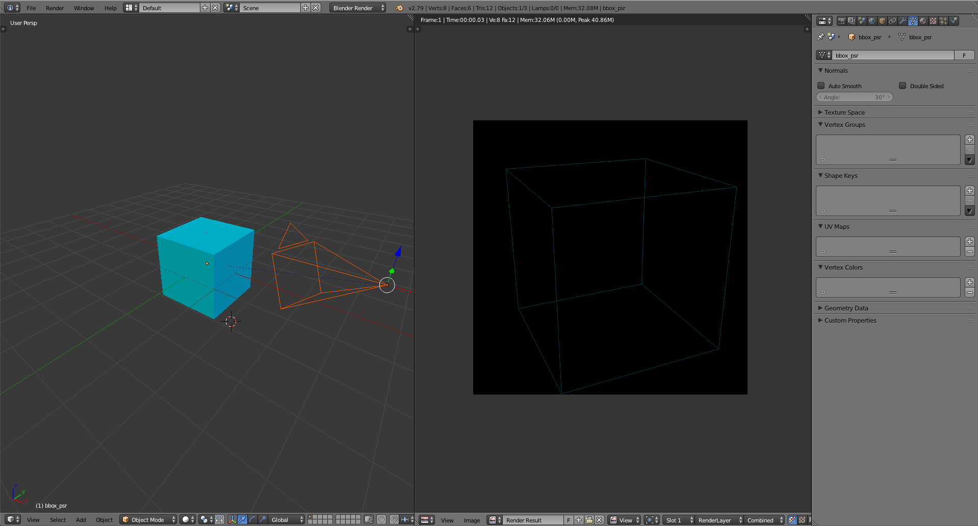
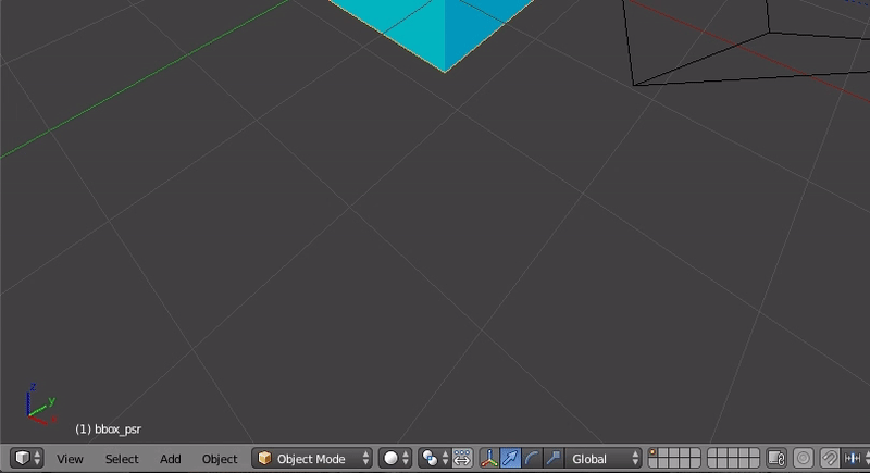
Bounding box¶

In some cases we’ll need a simple bounding box to make a 3D image more clear for perception. In BRender we can simply do:

bbox = br.BoundingBox(name = 'bbox')
bbox.size = [3.5, 1, 2] # <-- adjusting shape
bbox.location = [1, 0, 0] # <-- adjusting location
bbox.color = '#36b3c4' # <-- you can give color in any other format, e.g., (0.2, 0.34, 0.8) etc
bbox.intensity = 15. # <-- adjusting emission intensity of the bounding box

Note

I naturally prefer to keep everything simple, so all the visualization made in this module will be rescaled and plotted in the 2x2x2 cube (or with different aspect) centered in the (0,0,0).

Note

We can also change the material parameters from the GUI. The easiest way to do this is to access the material tab in the Properties and adjust the relevant numbers.

Creating a sphere¶

Sometimes it’s useful to visualize a simple object (such as a star) along with the simulation results to give a sense about the scales involved. In BRender you can do this by simply typing:

star = br.Sphere(name = 'my_star')
# then we can adjust location, color, size and emission intensity in the same fashion
star.size = (1.4, 1.4, 1.4)
star.location = (1, 0.4, -1)
star.intensity = 0.5

Running a script¶

If scripting in the Blender console doesn’t work for you, one can easily run a script written in the .py file with runScript() function:

br.runScript('/path-to-script/script.py')

Note

Be aware, that after a script is ran from the file you cannot directly access the objects from the console. Running a script like that is handy if you already have a tested code and you don’t want to copy+paste it to console every time you want to visualize new data.

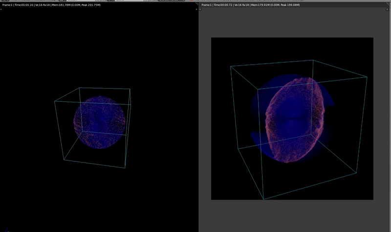
Interactive viewport¶

Sometimes when we need to briefly look at the render result from different angles to choose the right perspective, we can do this without actually rendering the image itself in a sort of interactive render regime.

To do this, activate Rendered viewport shading option in the 3D viewport as shown in the animation below.

The resulting interactive regime is shown below.