Volume plot
Before starting this section make sure to have a camera set up. Also if there’s a bounding box in the scene, it’s generally easier to navigate and understand the directions in space. So before moving forward, check previous tutorial on basics of BRender.
Note
for tigressdata users. Blender’s bundled python does not support hdf5 documents, and I wasn’t able to install it (no access). So you’ll have to do all the reading and primary analysis of all the data from some python outside Blender.
Generating VOXEL data
In general BRender is not constrained to any specific code output, and can be fed by any sort of Blender VOXEL (volumetric pixel) data file generated in advance. So if you know how to generate a .bvox file from a specific code output, feel free to skip to the next section where we’ll be making a volumetric plot.
Here we’ll discuss how to generate a .bvox file particularly for TRISTAN code output (hdf5 format), which will be later used to make a plot. Note again, that if you’re working from within the tigressdata, you’ll have to do this from a python outside Blender, Mac users can do this from inside Blender console. We first need to specify several paths and names:
# For tigressdata do this whole procedure from outside Blender python console
out_path = '/output-dir-for-bvox/' # <-- make sure to have slash in the end
fname = '/path-to/flds.tot.001' # <-- this one is specifically a TRISTAN output file
prefix = 'density' # <-- this is the prefix name of the file, in our case - density
Let’s say we want to plot a density. For that we specify a value function which takes the code data as an input and outputs the desired field in the correct form:
def valueFunc(data):
    return data['dens'].value # <-- we output whatever is under 'dens' key value
Note
If you don’t specify valueFunc() it will take a default function (which is just the 'dens' key).
Note
You could think of something more complicated, like a current density normalized by the distance to the center of the grid squared (this is relevant to pulsar magnetosphere simulations):
def valueFunc(data):
    sx, sy, sz = data['jx'].value.shape
    halfx, halfy, halfz = map(np.floor, np.array([sx, sy, sz]*0.5))
    rsquared = np.array([[[((x - halfx)**2 + (y - halfy)**2 + (z - halfz)**2) for x in range(sx)] for y in range(sy)] for z in range(sz)])
    return np.sqrt(np.array(data['jx'].value)**2 + np.array(data['jy'].value)**2 + np.array(data['jz'].value)**2) * rsquared
We can also specify a normalization function if we want (the default is just linear normalization):
def normalizeFunc(value):
    return np.log(1. + value) # <-- accepts real value and outputs normalized value
Other two options to specify are the maximum and minimum value. After the normalization, any value in the 3D grid above that maximum value and below the minimum will be diminished and set to the specified value:
min_val = 0.1 # <-- our function does the following val[val < min_val] = min_val
max_val = 0.8 # <-- our function does the following val[val > max_val] = max_val
Note
Default (in case you don’t specify) for min_val is 0, and for max_val is 1.
Ok, now with all those variables and functions specified, we are ready to output a .bvox file in the directory specified above:
import lib.to_bvox as bvox
bvoxfile = bvox.makeBvox(out_path, fname,
                            valueFunc = valueFunc,                      # optional
                            normalizeFunc = normalizeFunc,              # optional
                            min_val = min_val, max_val = max_val,       # optional
                            prefix = prefix)                            # optional
# now bvoxfile is a string containing the path to the generated `.bvox` file in case you need it
This might take some time, but you need to do this once to generate the .bvox file, later you can just refer to it with a full path to make plots.
Warning
For tigressdata you’ll first need to append sys.path when working outside Blender (add this at the start of code):
import sys
sys.path.append('/path-to-BRender-repo/') # you can use mine '/home/hakobyan/Downloads/brender_astro'
Also make sure you have h5py module loaded (in the terminal):
$ module load h5py27
Making volumetric plot
Finding the shape and scale
Since you’ll later need a shape of your simulation and scaling factor for your visualization, I’d suggest to do it right away with the following code:
# make sure to do 'import lib.to_bvox as bvox' as you probably did above
fname = '/path-to/flds.tot.001'
shape0 = np.array(bvox.getShape(fname, 'dens'))
scale = 2. / shape0.min()
shape = shape0 * scale
Now shape is a tuple of 3 float numbers with the normalized (size-x, size-y, size-z) of your data, and scale is a float number that determines how much is the original data “squeezed”. Again, tigressdata users can run this only outside Blender’s python.
Nailing the plot
Note
For tigressdata the rest can be done within the Blender console.
If you working within tigressdata, specify a path to .bvox file:
bvoxfile = '/path-to/dens.bvox'
You then can make an object that will have your volumetric plot:
density = br.VolumePlot(bvoxfile, name = 'my_density')
Note
If you later decide to redo your plot using a different .bvox file, there is no need to delete the object. Simply do:
density.voxdata = '/path-to-new/bvoxfile.bvox'
This will redo the plot only changing the volumetric pixel data provided (shape and other parameters will remain the same).
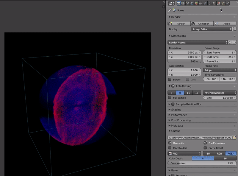
This creates a cube and fills it in according to voxel data. You can then work with this density object. By default the density is in 2x2x2 cube. We can adjust it by doing:
density.size = shape # <-- set the shape to already predefined
We can also adjust the colormap and brightness:
# let us first define a colormap
cmap = [[0.0, # <-- this is the position of the first color tag
            (0, 0, 1, 0)], # <-- this is the color in terms of (r, g, b, a)
        [0.7,
            (0, 0, 1, 0.3)],
        [0.86,
            (0.56, 0.878, 0.002, 0.8)],
        [1,
            (1, 0, 0, 1.0)]]
# ... and brightness
brightness = 0.6
density.cmap = cmap
density.brightness = brightness
Other more complex parameters to adjust are the density and contrast:
density.density = 5.
density.contrast = 0.35
Note
You can always play with those parameters (colormap, brightness, contrast, density, etc) from the Blender GUI (see below).
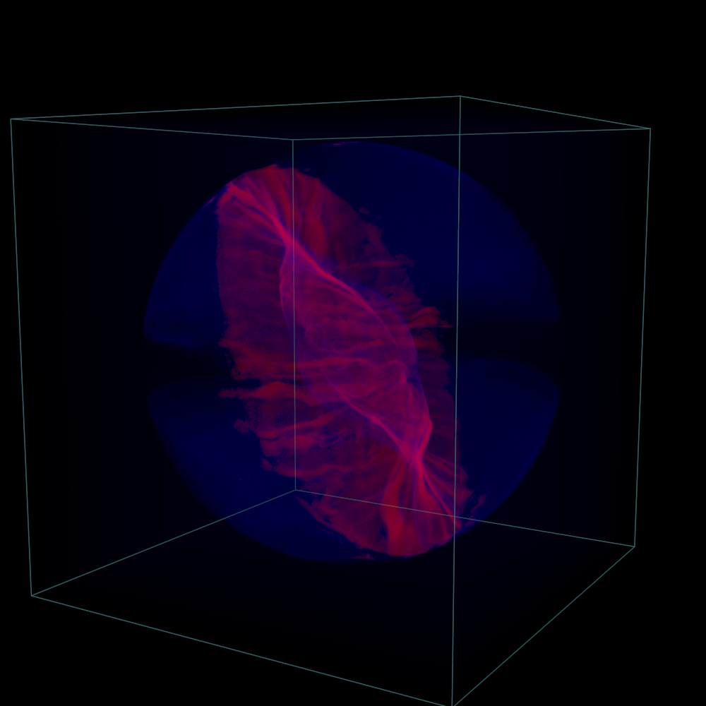
Below is a rendering result of such a plot.
Note
We can also enable the interactive viewport to look at the result from different angles on the fly (see here on how to do this).
Full python script
for Mac
"""Example code to run within Blender to produce the plot show above (Mac version)

    Note: Make sure to change all the paths below

"""

import brender as br

# # # # # # # # # # # # # # # # # # # # # # # #
#
#   1. Preparing
#
# # # # # # # # # # # # # # # # # # # # # # # #
# setting up the camera
cam = br.initializeCamera()
cam.location = (4.5, -1.2, 0.7)
cam.pointing = (0, 0, 0)

# setting up the renderer
render_directory = '/any-folder/images/'
render_name = 'mysim_'
render = br.Render(render_directory, render_name)

br.Render.set_resolution(1000, 1000)

import lib.to_bvox as bvox
import numpy as np

# finding the shape and scale of our simulation
fname = '/path-to/flds.tot.001' # <-- this is for TRISTAN
shape0 = np.array(bvox.getShape(fname, 'dens'))
scale = 2. / (shape0.min())
shape = shape0 * scale

# # # # # # # # # # # # # # # # # # # # # # # #
#
#   2. Generating .bvox file
#       if the .bvox already exists, just skip this step
#
# # # # # # # # # # # # # # # # # # # # # # # #
out_path = '/any-folder/bvoxfile/'

prefix = 'current'

# we will be plotting the |j|*R^2 for pulsar simulation
def valueFunc(data):
    sx = len(data['jx'].value[0][0])
    sy = len(data['jx'].value[0])
    sz = len(data['jx'].value)
    halfx = np.floor(sx/2.)
    halfy = np.floor(sy/2.)
    halfz = np.floor(sz/2.)
    rsquared = np.array([[[((x - halfx)**2 + (y - halfy)**2 + (z - halfz)**2)
                                for x in range(sx)]
                                for y in range(sy)]
                                for z in range(sz)])
    return np.sqrt(np.array(data['jx'].value)**2 + np.array(data['jy'].value)**2 + np.array(data['jz'].value)**2) * rsquared

# in log units
def normalizeFunc(value):
    return np.log(1. + value)

bvoxfile = bvox.makeBvox(out_path, fname,
                        valueFunc = valueFunc,
                        normalizeFunc = normalizeFunc,
                        max_val = 0.1,
                        prefix = prefix)

# now bvoxfile has the path to .bvox

# # # # # # # # # # # # # # # # # # # # # # # #
#
#   3. Plotting
#
# # # # # # # # # # # # # # # # # # # # # # # #
# generating the VolumePlot class object
density = br.VolumePlot(bvoxfile, name = 'my_current')

# adjusting shape, etc
density.size = shape
density.brightness = 1.1
density.contrast = 1.1
density.intensity = 10.
density.density = 3.

# making a bounding box
bbox = br.BoundingBox(name = 'bbox')

# adjusting parameters
bbox.size = shape
bbox.color = '#36b3c4'
bbox.intensity = 0.2

# ...and finally rendering (or use Fn+F12)
render.render()
# image saved to the directory defined above
for tigressdata
outside Blender:
"""Example code to run outside Blender (tigressdata version)

    Note: Make sure to change all the paths below
    Note2: This is to be run outside Blender

"""

import sys
sys.path.append('/path-to-brender-repo') # you can use mine: '/home/hakobyan/Downloads/brender_astro'
import lib.to_bvox as bvox

# # # # # # # # # # # # # # # # # # # # # # # #
#
#   1. Preparing
#
# # # # # # # # # # # # # # # # # # # # # # # #
fname = '/path-to/flds.tot.001'
shape0 = np.array(bvox.getShape(fname, 'dens'))
scale = 2. / (shape0.min())
shape = shape0 * scale

# you need to copy this parameters later
print (shape)
print (scale)

# # # # # # # # # # # # # # # # # # # # # # # #
#
#   2. Generating .bvox file
#       if the .bvox already exists, just skip this step
#
# # # # # # # # # # # # # # # # # # # # # # # #
out_path = '/any-folder/bvoxfile/'

prefix = 'current'

# we will be plotting the |j|*R^2 for pulsar simulation
def valueFunc(data):
    sx = len(data['jx'].value[0][0])
    sy = len(data['jx'].value[0])
    sz = len(data['jx'].value)
    halfx = np.floor(sx/2.)
    halfy = np.floor(sy/2.)
    halfz = np.floor(sz/2.)
    rsquared = np.array([[[((x - halfx)**2 + (y - halfy)**2 + (z - halfz)**2)
                                for x in range(sx)]
                                for y in range(sy)]
                                for z in range(sz)])
    return np.sqrt(np.array(data['jx'].value)**2 + np.array(data['jy'].value)**2 + np.array(data['jz'].value)**2) * rsquared

# in log units
def normalizeFunc(value):
    return np.log(1. + value)

bvoxfile = bvox.makeBvox(out_path, fname,
                        valueFunc = valueFunc,
                        normalizeFunc = normalizeFunc,
                        max_val = 0.1,
                        prefix = prefix)
inside Blender:
"""Example code to run inside Blender (tigressdata version)

    Note: Make sure to change all the paths below
    Note2: This is to be run inside Blender, we do not refer to h5py here

"""

# # # # # # # # # # # # # # # # # # # # # # # #
#
#   1. Preparing
#
# # # # # # # # # # # # # # # # # # # # # # # #
# setting up the camera
cam = br.initializeCamera()
cam.location = (4.5, -1.2, 0.7)
cam.pointing = (0, 0, 0)

# setting up the renderer
render_directory = '/any-folder/images/'
render_name = 'mysim_'
render = br.Render(render_directory, render_name)

br.Render.set_resolution(1000, 1000)

# # # # # # # # # # # # # # # # # # # # # # # #
#
#   2. Plotting
#
# # # # # # # # # # # # # # # # # # # # # # # #
# generating the VolumePlot class object
bvoxfile = '/path-to-saved/bvoxfile.bvox'
density = br.VolumePlot(bvoxfile, name = 'my_current')

# adjusting shape, etc
density.size = [...] # <-- set by hands from the print output above
density.brightness = 1.1
density.contrast = 1.1
density.intensity = 10.
density.density = 3.

# making a bounding box
bbox = br.BoundingBox(name = 'bbox')

# adjusting parameters
bbox.size = shape
bbox.color = '#36b3c4'
bbox.intensity = 0.2

# ...and finally rendering (or use Fn+F12)
render.render()
# image saved to the directory defined above